Follow Us

My Fun Blog :: Google Blog :: Fun Img Post :: Twitter Post

Google

Fwd: MS EXCEL: AUTOMATICALLY ALTERNATE ROW COLORS (ONE SHADED, ONE WHITE) IN EXCEL 2003

MS EXCEL: AUTOMATICALLY ALTERNATE ROW COLORS (ONE SHADED, ONE WHITE) IN EXCEL 2003

How can I set up alternating row colors in Microsoft Excel 2003. I don't want to have to change the row colors every time I insert, delete, or move a row.

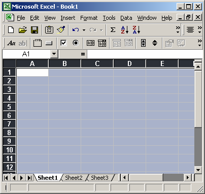
Answer: If you wish to set up alternating row colors in Excel, first highlight the rows that you wish to apply the formatting to. In this example, we've selected all rows in the spreadsheet.

Microsoft Excel

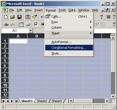
Under the Format menu, select Conditional Formatting.

Microsoft Excel

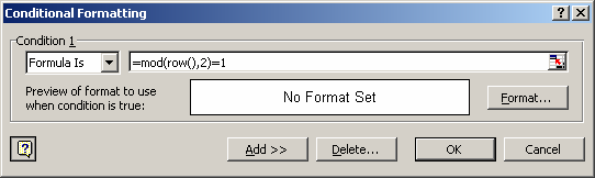
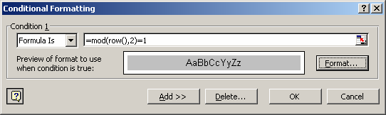
When the Conditional Formatting window appears, select "Formula Is" in the drop down. Then enter the following formula:

=mod(row(),2)=1

Next, we need to select the color we want to see in the alternating rows. To do this, click on the Format button.

Microsoft Excel

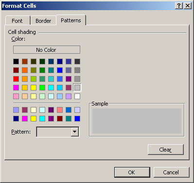
When the Format Cells window appears, select the Patterns tab. Then select the color that you'd like to see. In this example, we've selected a light grey. Then click on the OK button.

Microsoft Excel

When you return to the Conditional Formatting window, you should see the following. Next, click on the OK button.

Microsoft Excel

Now when you return to the spreadsheet, the conditional formatting will be applied.

As you can see, you now have alternating colors in the rows. You can insert, delete, and move rows, and you don't have to worry about reapplying formatting.

Microsoft Excel

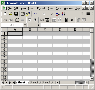
What a wonderful formatting trick!

Fwd: Transpose a Values in a Row to Column using Formulas - In Excel

Transpose a values in a row to column using formulas When entering data for credit cards, I use one column per card. But in my report view, I want to show credit card details in rows. How do I do this? Something like this:


Transposing values in a row to column using formulas

If it is a onetime process, my friend can use Paste Special > Transpose feature and be done. But this is no one time business. So lets understand which formula helps us do this.

1.       Lets assume original data is in $F$4:$J$5. Row 4 has card names & Row 5 has amounts.

2.       Wherever you want the out put, just list running numbers (1,2,3….) in a column. Lets say these are in cells D10:D14.

3.       To get the first card name, you can use the formula =INDEX($F$4:$J$4, $D10).

4.        To get the first amount due, use the formula =INDEX($F$5:$J$5, $D10)

5.       Now drag both these formulas down and you are done!

This is good, but I don’t like the extra column…

If that is the case, you can use the ROWS() formula to generate these running numbers for you on the fly. For example,

=INDEX($F$4:$J$4, ROWS($A$1:A1)) would work perfectly.

Visitor Comments

Subscribe via email

Enter your email address:

Delivered by FeedBurner

Twitter